Start

Begin

At the beginning of whole analysis, you need to finish installing the MATLAB(you could see a lot of tutorial on website whatever it’s Cracked or Genuine) and know some basic programming language.

Toolbox Download

Then you need to download the MATLAB toolbox of Dynamic Copula Toolbox 3.0, you could click here, and then put it into your workspace.

Preparation

First of all, you need to import your data from excel or other files, and named the variable like data or any other names, then remember it.

Secondly, you should click twice on the Dynamic Copula Toolbox folder and enter this, then you could start your analysis.

Process

Then you could enter the command into the terminal of MATLAB, following with my step.

Now, you could enter this command into the terminal below.

1

spec = modelspec(data)

Then you’ll see the window like this.

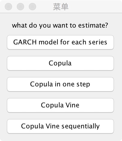
Choose “Garch model for each series”, and it will start to estimate the Garch model for marginal distribution.

Then you would see the output like this.

If these series have autocorrelation, you should enter “1”, but if they don’t, just enter “0” is enough.

Then press the keyboard “enter”, it’ll continue, and the window like this will appear.

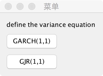
You should choose a model for what you want, and click it. Then it’ll go to the next period.

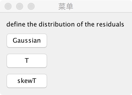
If you see this, you’ll fell a bit close. It’s the distribution of residuals, you just need to choose the fittest one. Even though the Skew T and T is the most general. Choose it and click it!

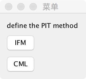
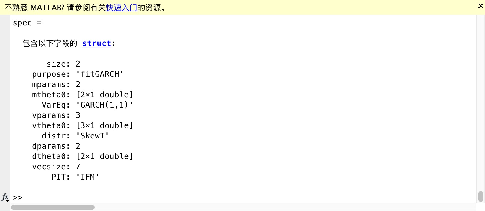
Then you’ll see this window, the IFM means Two-Stage Maximum Likelihood Estimation, I think it is more general, and you’ll see the configuration in the command window.

Then you need to input the next command.

1

[parameters, LogL, evalmodel, GradHess, varargout] = fitModel(spec, data, 'fmincon')

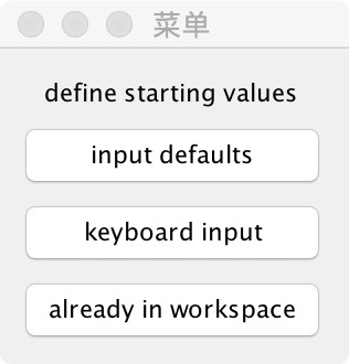
After running, you could see a window appear.

As for me, it’s really enough to click the “input defaults”, then the terminal will start running and the window below will become a few seconds later.

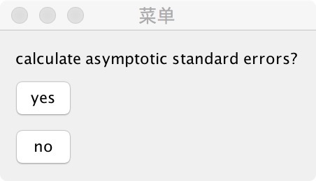
Generally, you could click yes for the estimation of standard errors.

Then the estimate result would be there.

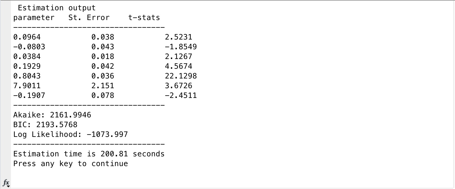
You just need to press enter then it’ll be going on. The second same window will appear soon, you just need to click “yes” again and the estimation is done.

Of course, it’s a good chance for you to save the variable and you should input the code below to do this.

1
2
3
4

[LogL, LL, ht, stdRes, udata]=GARCHLogL(parameters(:,[1]),data(:,[1]),spec, 'fmincon')
ht1=ht
[LogL, LL, ht, stdRes, udata]=GARCHLogL(parameters(:,[2]),data(:,[2]),spec, 'fmincon')
ht2=ht

Now the variable varargout is the standard deviation probability residual integral transforms the sequence that follows for Garch model.

You’d like to start the copula model with this variable.

Just input this code into the terminal.

1

spec=modelspec(varargout)

It’ll start estimate for Copula Model and you’ll see the same window again.

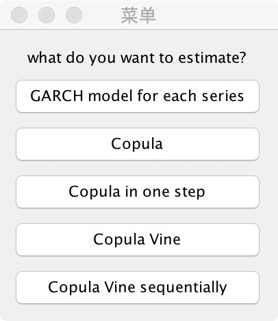
But at this time, you should click “Copula” and the window below would happen.

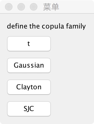
You could choose the copula family you want, just click it and you will see another window.

You can decide which style you need, the “static” means stable type, and the “DCC” means the dynamic type.

After clicking, you will see the configuration of copula estimation on command window, then you need to input the code below and it’s the last step.

1

[parameters, LogL, evalmodel, GradHess, varargout] = fitModel(spec, varargout, 'fmincon')

You’ll see it again and just choose “input defaults”.

Then it has started to estimate and you can choose if you need to calculate the standard errors and click “yes”, the whole process is completed.

You can calculate the $VaR$, $CoVaR$, $\Delta CoVar$ at this time, here are some commands to help you calculate them.

1
2
3
4
5
6

var1=norminv(0.95)*sqrt(ht1)
var12=norminv(0.05)*sqrt(ht1)
covar121=norminv(0.95)*sqrt(ht2).*sqrt(1-evalmodel.Rt.^2)+norminv(0.05)*evalmodel.Rt.*sqrt(ht1) 
covar122=norminv(0.05)*sqrt(ht2).*sqrt(1-evalmodel.Rt.^2)+norminv(0.05)*evalmodel.Rt.*sqrt(ht1) 
covar123=norminv(0.05)*sqrt(ht2).*sqrt(1-evalmodel.Rt.^2)+norminv(0.95)*evalmodel.Rt.*sqrt(ht1) 
covar124=norminv(0.95)*sqrt(ht2).*sqrt(1-evalmodel.Rt.^2)+norminv(0.95)*evalmodel.Rt.*sqrt(ht1) 

The dynamic correlation coefficient is in the Rt of evalmodel and the parameters variable includes the copula parameters that it estimated just now.

You could also to draw it like the figure below.

Lastly, you could calculate the $\Delta CoVaR$ by MATLAB easily and the code I provided below might help you.

1
2
3
4

dcovar121=norminv(0.95)*evalmodel.Rt.*sqrt(ht1) 
dcovar122=norminv(0.05)*evalmodel.Rt.*sqrt(ht1) 
dcovar211=norminv(0.95)*evalmodel.Rt.*sqrt(ht2) 
dcovar212=norminv(0.05)*evalmodel.Rt.*sqrt(ht2) 

The picture always looks like this.

At last, I don’t know why I didn’t find any usefull information about this toolbox on the website and in some places, even need to spend money on these code, so I think my work would help some people who also feel annoyed like me when they are researching the dynamic copula model.